Configure — Choose the Level of Theory
Configure your calculation — first pick a compute backend (Classical · PySCF, Classical · ORCA, Quantum, or ML potential · MACE), then the method, basis set, and solvation model, plus optional properties and tuning. Classical work runs through PySCF or, if you have your own licensed copy installed, ORCA; the quantum side offers a dozen eigensolvers plus vibrational-structure and open-system dynamics on the engine's local statevector simulator (OpenFermion operator algebra; Qiskit is needed only for circuit export and IBM hardware), most with an optional real gate-circuit path; the MACE backend runs machine-learned interatomic potentials as a fast DFT surrogate. A live script preview and inline validation show exactly what will run before you submit.
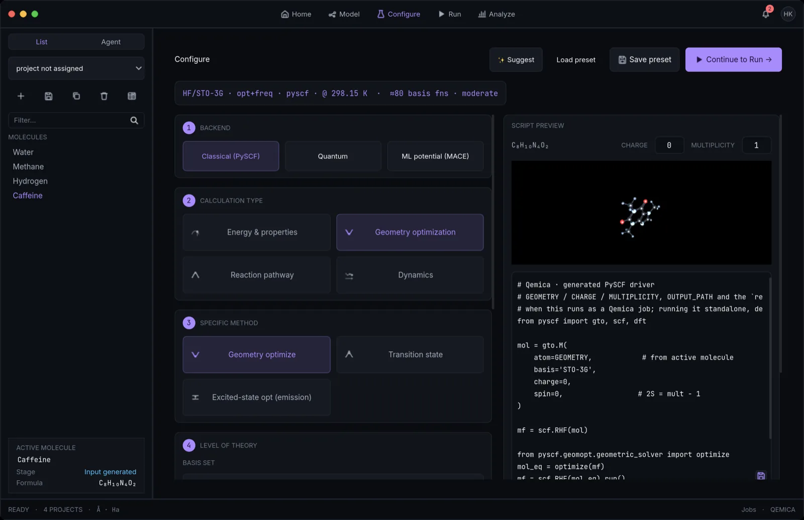
Calculation types
- Single-point energy — energy and properties (charges, dipole, orbitals) at a fixed geometry.
- Geometry optimize — relax the structure to a minimum.
- Frequencies (IR) — vibrational frequencies, IR intensities, Raman scattering, and thermochemistry (H, S, G) at an editable temperature and pressure (defaults 298.15 K, 1 atm).
- Optimize + frequencies — optimization followed by a frequency analysis at the minimum.
- Transition state and IRC — locate a first-order saddle point (confirmed by one imaginary mode) and trace the intrinsic reaction coordinate to reactants and products.
- NEB (reaction path) — a nudged-elastic-band chain of images from reactant to product, giving the minimum-energy path and barrier with a climbing-image saddle estimate.
- Relaxed scan — drive a distance, angle, or dihedral through a range, re-optimizing everything else at each point for a true reaction-energy profile.
- Molecular dynamics — propagate atoms under computed forces (velocity-Verlet) at your chosen temperature.
- Excited states (UV-Vis) and Excited-state opt (emission) — vertical transition energies and oscillator strengths via TDA/TDDFT, or relaxation on the excited-state gradient.
Method, functional, and basis set
Choose the wavefunction theory, then (for DFT) a functional and an atomic-orbital basis. The recipe pill summarizes your choices, for example 'B3LYP/def2-SVP · optimize · pyscf · D3(BJ)'.
- Classical methods (Classical · PySCF): HF, DFT, MP2 and CCSD (energy and geometry optimization on analytic gradients), CCSD(T) and FCI (single-point energy — FCI is exact and capped to small systems), and CASSCF (multi-configurational; pick the active space in Analyze → Surfaces). Post-HF honesty: solvation is treated at the SCF reference (warned in the result), and empirical dispersion is refused for post-HF methods rather than double-counting correlation. The full quantum method set (VQE, ADAPT-VQE, CQE, SQD, QPE, QCELS, RPE, QMEGS, BPE, BPDE, QKD, QAAE, plus vibrational and open-system dynamics) lives under the Quantum backend — see the quantum panel below.
- Classical methods (Classical · ORCA): the same set bar FCI — HF, DFT, MP2, CCSD, CCSD(T) and CASSCF — across every calculation type the classical side offers (energy, optimize, frequencies, opt+freq, transition state, IRC, NEB, relaxed scan, excited states, excited-state opt, MD), with CPCM and SMD solvation and D3/D4 dispersion. Qemica renders the .inp file and you can edit it before submitting; it runs exactly what the preview shows. Two things stay on PySCF: FCI, and the Fukui and NBO-style bonding analyses, which Qemica computes from the wavefunction itself.
- DFT functionals by Jacob's Ladder: GGA (BLYP, BP86, PBE, revPBE, B97-D), meta-GGA (TPSS, TPSSh, SCAN, r2SCAN, M06-L), hybrid (B3LYP, B3PW91, PBE0, M06, M06-2X), and range-separated (CAM-B3LYP, ωB97X-V, ωB97M-V). ωB97X-D is deliberately not offered: PySCF does not implement its −D2 dispersion term, so running it would compute plain ωB97X — a different, dispersion-free functional — under the name you asked for. ωB97X-V and ωB97M-V carry dispersion through the nonlocal VV10 term, which is fully evaluated here.
- Frozen core: MP2, CCSD and CCSD(T) freeze the atomic-core orbitals by default, matching Gaussian, ORCA and Q-Chem — essentially every published post-HF number is frozen-core, and correlating the core in a valence correlation-consistent basis (cc-pVXZ, def2) is unbalanced. Each result records which convention it used.
- Basis sets: minimal (STO-3G, 3-21G), standard Pople (6-31G(d) through 6-311++G(d,p)), polarized def2 (def2-SVP/TZVP/QZVP), and correlation-consistent Dunning (cc-pVDZ through aug-cc-pVTZ).
- Custom basis and ECP: pick Custom… in the basis dropdown to type any PySCF basis string — including a per-element assignment — plus an optional effective core potential (e.g. lanl2dz for heavy elements). Strings PySCF does not recognize are rejected at submit with the engine's own error.
- Dispersion: None, D3, D3(BJ), or D4 (Grimme).
- Tip: Start with 6-31G(d) or def2-SVP; for charge-transfer excitations use a range-separated functional (CAM-B3LYP, ωB97X-V) since standard hybrids underestimate CT energies.
- Tip — anions and excited states need diffuse functions: an added electron, and any Rydberg or charge-transfer state, is spatially diffuse and simply cannot be described without them. Use 6-31+G(d), 6-311++G(d,p), aug-cc-pVDZ or def2-TZVPD. Qemica warns when you run an anion in a basis with no diffuse set, and when excited states come back above the ionization threshold — the energy error there runs to tens of kcal/mol.
Quantum methods — the compute-backend choice and the quantum panel
Pick the compute backend at the top of Configure: Classical (PySCF), Classical (ORCA), Quantum, or ML potential (MACE). Choosing Quantum swaps in a panel of quantum options (the basis set is shared with the classical side). Everything runs on the engine's local statevector simulator (no Qiskit required) unless you target IBM Quantum hardware in Run. The full algorithm list and the gate-circuit option are described in the Quantum Computing section below.
- Algorithm: a dozen eigensolvers — VQE (UCCSD), ADAPT-VQE, CQE, SQD, QPE, and the short-depth signal/Krylov family (QCELS, RPE, QMEGS, BPE, BPDE, QKD, QAAE) — plus the Vibrational (quantum) and Open-system dynamics calc types. Algorithms with no faithful IBM-hardware path carry a warning glyph on their chip.
- Gate-circuit option: for most methods, a toggle runs the method as a real universal-gate circuit (Qiskit-exportable with the optional Qiskit components) instead of the exact dense path; the exact path stays the default.
- Qubit mapping: Jordan–Wigner or Bravyi–Kitaev (OpenFermion interleaved spin ordering); both run end-to-end. Parity mapping is not offered.
- Hamiltonian formulation: optional frozen core (drop chemically-inert core orbitals) and an explicit active space (active orbitals / electrons) to shrink the qubit Hamiltonian.
- Shots: applies on the IBM Quantum hardware target (chosen in Run); the local simulator is exact (statevector), so shots do not change a local result.
- Per-method tuning: VQE/ADAPT optimizer (COBYLA default, SLSQP, L-BFGS-B, Nelder-Mead, Powell, SPSA), iterations, tolerance/gradient threshold; QPE ancilla bits and Trotter steps; per-family sample/round/dissipator controls.
- A live estimate shows the circuit width (qubits) and an approximate depth as you change options, so you see the cost before you run.
- Guardrails: ground-state energy methods run as a single-point; open shells are supported on a restricted-open (ROHF) reference — the active space must be physical and hold every unpaired electron (validated before submit); and an oversized circuit is blocked before it exceeds the local simulator (≈20 qubits for VQE, ≈12 system qubits for the dense time-evolution methods).
ML potential (MACE) — a fast DFT surrogate
The third backend runs MACE machine-learned interatomic potentials — DFT-quality energies and forces at a fraction of the cost, ideal for larger systems, conformer sweeps, MD, and reaction-path prescreens before a full quantum treatment.
- Foundation models: MACE-OFF small/medium/large for organic molecules (covering H, B, C, N, O, F, Si, P, S, Cl, Br, I) and MACE-MP-0 for materials (~89 elements); you can also load your own fine-tuned checkpoint file.
- Calc types served: single-point, geometry optimize, frequencies, opt+freq, MD, NEB, IRC, and relaxed scan — dispatched through the same energy/gradient machinery as PySCF.
- Compute device: CPU, CUDA (NVIDIA GPU), or MPS (Apple Silicon GPU), with selectable float precision; a committee of models can report a per-prediction uncertainty spread.
- Capability-gated: the MACE card is greyed until torch + ase + mace-torch are installed — one click on the capability pill under Config → Engines.
Solvation, charge, and multiplicity
- Solvation models: Gas phase, C-PCM, IEF-PCM, SMD (offered when the engine build supports it), or COSMO (run as ddCOSMO). When active, choose from 22 named solvents (water, DMSO, acetonitrile, methanol, dichloromethane, THF, toluene, and more) or a Custom entry with a manually entered dielectric constant ε — custom ε works with C-PCM/IEF-PCM/COSMO; SMD needs a named solvent's full descriptor set.
- Charge: net electronic charge (−10 to +10); 0 neutral, +1 cation, −1 anion.
- Multiplicity: 2S+1 — 1 for a closed-shell singlet, 2 for a doublet radical, 3 for a triplet (e.g. neutral O₂). Both are seeded from the molecule and editable here.
Optional properties and engine-specific tuning
Opt-in properties add compute time but run within a single job. Additional controls appear for the relevant calc type or method.
- Properties: volumetric surfaces (orbital/density/ESP .cube files), NMR shieldings (GIAO), static polarizability, Fukui reactivity indices (cost two extra SCFs), and localized-bonding (NBO-style) analysis for the Bonding tab.
- Excited states: TDA (default, faster) or TDDFT, number of states (default 5), triplet manifold, and optional Natural Transition Orbitals.
- MD: integration steps (default 20) and temperature (default 300 K). Scans: coordinate kind, 0-indexed atom indices, and From/To/Steps.
- Quantum tuning (algorithm, mapping, Hamiltonian formulation, optimizer, ancilla/Trotter) lives in the Quantum panel above — see 'Quantum methods'.
- Periodic systems (PBC): a k-points Monkhorst–Pack mesh; periodic runs use GTH pseudopotentials and the GTH-SZV basis.
- Geometry constraints: bonds, angles, or dihedrals frozen in Model (Measure → Freeze) are honored by the optimizer and recorded in provenance.
Resources, presets, and submit
- Resources: CPU cores (1–64, default 4) and memory (1–256 GB, default 8). Insufficient memory causes an out-of-core failure.
- ✨ Suggest — a guided methodology wizard: answer three short questions about your goal, and hardware-aware ranked recipe cards appear; pick one and Confirm to apply the whole recipe (calc type, method, functional, basis) in one click.
- Presets: built-in starters include 'HF energy — STO-3G', 'DFT geometry opt — B3LYP-D3(BJ)/def2-SVP', and 'VQE — STO-3G'; save your own with the Save preset button.
- Editable script: the live Script preview is genuine — every line reflects what the engine will execute — and it is editable. Hand-edit it and exactly that script runs on submit instead of the generated one.
- Export it: the preview's save button writes a standalone-runnable .py — python <file> in a terminal (against your engine environment) reproduces the in-app result and writes result.json; pasting it back into the preview still runs identically as a job.
- Validation: a panel flags incompatible combinations (e.g. multiplicity/charge mismatch) in red; Continue to Run enables only when the recipe is valid and a molecule is loaded.
- Continue to Run carries the composed recipe to the Run screen, where Submit dispatches it to the queue.
References
- B3LYPBecke, J. Chem. Phys. 98, 5648 (1993); Lee, Yang & Parr, Phys. Rev. B 37, 785 (1988)
- B88 / P86 (BLYP, BP86)Becke, Phys. Rev. A 38, 3098 (1988); Perdew, Phys. Rev. B 33, 8822 (1986)
- PBEPerdew, Burke & Ernzerhof, Phys. Rev. Lett. 77, 3865 (1996)
- PBE0Adamo & Barone, J. Chem. Phys. 110, 6158 (1999)
- B97-DGrimme, J. Comput. Chem. 27, 1787 (2006)
- M06 familyZhao & Truhlar, Theor. Chem. Acc. 120, 215 (2008); Zhao & Truhlar, J. Chem. Phys. 125, 194101 (2006)
- CAM-B3LYPYanai, Tew & Handy, Chem. Phys. Lett. 393, 51 (2004)
- ωB97X-DChai & Head-Gordon, Phys. Chem. Chem. Phys. 10, 6615 (2008)
- SCANSun, Ruzsinszky & Perdew, Phys. Rev. Lett. 115, 036402 (2015)
- r²SCANFurness, Kaplan, Ning, Perdew & Sun, J. Phys. Chem. Lett. 11, 8208 (2020)
- TPSSTao, Perdew, Staroverov & Scuseria, Phys. Rev. Lett. 91, 146401 (2003)
- Pople basis setsHehre, Stewart & Pople, J. Chem. Phys. 51, 2657 (1969); Hehre, Ditchfield & Pople, J. Chem. Phys. 56, 2257 (1972); Krishnan, Binkley, Seeger & Pople, J. Chem. Phys. 72, 650 (1980)
- def2 basisWeigend & Ahlrichs, Phys. Chem. Chem. Phys. 7, 3297 (2005)
- cc-pVXZ basisDunning, J. Chem. Phys. 90, 1007 (1989); Kendall, Dunning & Harrison, J. Chem. Phys. 96, 6796 (1992)
- LANL2DZ ECPHay & Wadt, J. Chem. Phys. 82, 270 (1985)
- DFT-D3Grimme, Antony, Ehrlich & Krieg, J. Chem. Phys. 132, 154104 (2010)
- D3(BJ)Grimme, Ehrlich & Goerigk, J. Comput. Chem. 32, 1456 (2011)
- DFT-D4Caldeweyher, Ehlert, Hansen, et al., J. Chem. Phys. 150, 154122 (2019)
- PCMMiertuš, Scrocco & Tomasi, Chem. Phys. 55, 117 (1981); Tomasi, Mennucci & Cammi, Chem. Rev. 105, 2999 (2005)
- COSMOKlamt & Schüürmann, J. Chem. Soc., Perkin Trans. 2, 799 (1993)
- MP2Møller & Plesset, Phys. Rev. 46, 618 (1934)
- CCSDPurvis & Bartlett, J. Chem. Phys. 76, 1910 (1982)
- CCSD(T)Raghavachari, Trucks, Pople & Head-Gordon, Chem. Phys. Lett. 157, 479 (1989)
- CASSCFRoos, Taylor & Siegbahn, Chem. Phys. 48, 157 (1980)
- TDDFTRunge & Gross, Phys. Rev. Lett. 52, 997 (1984); Casida, in Recent Advances in Density Functional Methods, Part I, 155 (1995)
- TDAHirata & Head-Gordon, Chem. Phys. Lett. 314, 291 (1999)
- ωB97M-VMardirossian & Head-Gordon, J. Chem. Phys. 144, 214110 (2016)
- GIAO (NMR)Ditchfield, Mol. Phys. 27, 789 (1974); Wolinski, Hinton & Pulay, J. Am. Chem. Soc. 112, 8251 (1990)
- NEB (climbing image)Henkelman & Jónsson, J. Chem. Phys. 113, 9978 (2000); Henkelman, Uberuaga & Jónsson, J. Chem. Phys. 113, 9901 (2000)
- Velocity Verlet (MD)Verlet, Phys. Rev. 159, 98 (1967); Swope, Andersen, Berens & Wilson, J. Chem. Phys. 76, 637 (1982)
- Monkhorst–Pack k-pointsMonkhorst & Pack, Phys. Rev. B 13, 5188 (1976)
- GTH pseudopotentialsGoedecker, Teter & Hutter, Phys. Rev. B 54, 1703 (1996); Hartwigsen, Goedecker & Hutter, Phys. Rev. B 58, 3641 (1998)
- geomeTRICWang & Song, J. Chem. Phys. 144, 214108 (2016)
- MACEBatatia, Kovács, Simm, Ortner & Csányi, NeurIPS 35 (2022), arXiv:2206.07697
- MACE-OFFKovács, Moore, Browning, Batatia, et al., arXiv:2312.15211 (2023)
- MACE-MP-0Batatia, Benner, Chiang, Elena, et al., arXiv:2401.00096 (2024)